인공지능

[밑바닥부터 시작하는 딥러닝] Part_1/CHAPTER 3 신경망/CHAPTER 3 신경망

SBOX Learning by doing 2022. 7. 23. 16:09

밑바닥 부터 시작하는 딥러닝

계단 함수 구현하기

In [3]:

import numpy as np
x = np.array([-1.0, 1.0, 2.0])
x

Out[3]:

array([-1.,  1.,  2.])

In [4]:

y = x > 0
y

Out[4]:

array([False,  True,  True])

In [5]:

y = y.astype(np.int)
y

Out[5]:

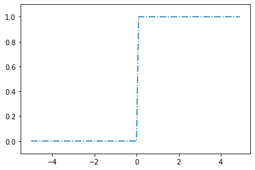
array([0, 1, 1])

계단함수의 그래프

In [18]:

import numpy as np
import matplotlib.pylab as plt

def step_function(x):
    return np.array(x > 0, dtype = np.int)

x = np.arange(-5.0, 5.0, 0.1)
y = step_function(x)
plt.plot(x,y,'-.')
plt.ylim(-0.1, 1.1) # y축의 범위 지정
plt.show()

시그모이드 함수 구현하기

In [7]:

def sigmoid(x):
    return 1 / (1 + np.exp(-x))

In [8]:

x = np.array([-1.0, 1.0, 2.0])

In [9]:

sigmoid(x)

Out[9]:

array([0.26894142, 0.73105858, 0.88079708])

In [12]:

x = np.arange(-5.0, 5.0, 0.1)
y = sigmoid(x)
plt.plot(x,y)
plt.ylim(-0.1, 1.1) # y축의 범위 지정
plt.show()

ReLU함수

In [19]:

def relu(x):
    return np.maximum(0, x)

In [20]:

x = np.array([-1.0, 1.0, 2.0])

In [21]:

relu(x)

Out[21]:

array([0., 1., 2.])

In [24]:

x = np.arange(-5.0, 5.0, 0.1)
y = relu(x)
plt.plot(x,y)
plt.show()

다차원 배열의 계산

다차원 배열

In [26]:

import numpy as np
A = np.array([1, 2, 3, 4])
print(A)

[1 2 3 4]

In [27]:

np.ndim(A)

Out[27]:

In [28]:

A.shape

Out[28]:

(4,)

In [30]:

A.shape[0]

Out[30]:

In [31]:

B = np.array([[1, 2], [3, 4], [5, 6]])
print(B)

[[1 2]
 [3 4]
 [5 6]]

In [32]:

np.ndim(B)

Out[32]:

In [33]:

B.shape

Out[33]:

(3, 2)

행렬의 곱

In [34]:

A = np.array([[1, 2], [3, 4]])
A.shape

Out[34]:

(2, 2)

In [35]:

B = np.array([[5, 6], [7, 8]])
B.shape

Out[35]:

(2, 2)

In [36]:

np.dot(A, B)

Out[36]:

array([[19, 22],
       [43, 50]])

In [37]:

A = np.array([[1, 2, 3], [4, 5, 6]])
A.shape

Out[37]:

(2, 3)

In [38]:

B = np.array([[1, 2], [3, 4], [5, 6]])
B.shape

Out[38]:

(3, 2)

In [39]:

np.dot(A, B)

Out[39]:

array([[22, 28],
       [49, 64]])

In [40]:

C = np.array([[1, 2], [3, 4]])
C.shape

Out[40]:

(2, 2)

In [41]:

A.shape

Out[41]:

(2, 3)

In [42]:

np.dot(A, C)

---------------------------------------------------------------------------
ValueError                                Traceback (most recent call last)
<ipython-input-42-bb5afb89b162> in <module>
----> 1 np.dot(A, C)

<__array_function__ internals> in dot(*args, **kwargs)

ValueError: shapes (2,3) and (2,2) not aligned: 3 (dim 1) != 2 (dim 0)

신경망에서의 행렬 곱

In [43]:

X = np.array([1, 2])
X.shape

Out[43]:

(2,)

In [44]:

W = np.array([[1, 3, 5],[2, 4, 6]])
print(W)

[[1 3 5]
 [2 4 6]]

In [47]:

W.shape

Out[47]:

(2, 3)

In [46]:

Y = np.dot(X, W)
print(Y)

[ 5 11 17]

각 층의 신호 전달 구현하기

In [50]:

X = np.array([1.0, 0.5])
W1 = np.array([[0.1, 0.3, 0.5], [0.2, 0.4, 0.6]])
B1 = np.array([0.1, 0.2, 0.3])

print(W1.shape) # (2, 3)
print(X.shape)  # (2,)
print(B1.shape) # (3,)

A1 = np.dot(X, W1) + B1
Z1 = sigmoid(A1)

print(A1)
print(Z1)

(2, 3)
(2,)
(3,)
[0.3 0.7 1.1]
[0.57444252 0.66818777 0.75026011]

In [55]:

W2 = np.array([[0.1, 0.4], [0.2, 0.5], [0.3, 0.6]])
B2 = np.array([0.1, 0.2])

print(Z1.shape) 
print(W2.shape) 
print(B2.shape) 

A2 = np.dot(Z1, W2) + B2
Z2 = sigmoid(A2)

(3,)
(3, 2)
(2,)

In [58]:

def identity_function(x):
    return x

W3 = np.array([[0.1, 0.3], [0.2, 0.4]])
B3 = np.array([0.1, 0.2])

A3 = np.dot(Z2, W3) + B3
Y = identity_function(A3)

In [64]:

def init_network():
    network = {}
    network['W1'] = np.array([[0.1, 0.3, 0.5], [0.2, 0.4, 0.6]])
    network['b1'] = np.array([0.1, 0.2, 0.3])
    network['W2'] = np.array([[0.1, 0.4], [0.2, 0.5], [0.3, 0.6]])
    network['b2'] = np.array([0.1, 0.2])
    network['W3'] = np.array([[0.1, 0.3], [0.2, 0.4]])
    network['b3'] = np.array([0.1, 0.2])
    return network

def forward(network, x):
    W1, W2, W3 = network['W1'], network['W2'], network['W3']
    b1, b2, b3 = network['b1'], network['b2'], network['b3']
    
    a1 = np.dot(x, W1) + b1
    z1 = sigmoid(a1)
    a2 = np.dot(z1, W2) + b2
    z2 = sigmoid(a2)
    a3 = np.dot(z2, W3) + b3
    y = identity_function(a3)
        
    return y

network = init_network()
x = np.array([1.0, 0.5])
y = forward(network, x)
print(y)

[0.31682708 0.69627909]

항등 함수와 소프트맥스 함수 구현하기

In [65]:

a = np.array([0.3, 2.9, 4.0])

exp_a = np.exp(a)
print(exp_a)

[ 1.34985881 18.17414537 54.59815003]

In [67]:

sum_exp_a = np.sum(exp_a)
print(sum_exp_a)

74.1221542101633

In [68]:

y = exp_a / sum_exp_a
print(y)

[0.01821127 0.24519181 0.73659691]

In [69]:

def softmax(a):
    exp_a = np.exp(a)
    sum_exp_a = np.sum(exp_a)
    y = exp_a / sum_exp_a
    
    return y

In [73]:

def softmax(a):
    c = np.max(a)
    exp_a = np.exp(a - c) # 오버플로 대책
    sum_exp_a = np.sum(exp_a)
    y = exp_a / sum_exp_a
    return y

In [74]:

a = np.array([0.3, 2.9, 4.0])
y = softmax(a)
print(y)

[0.01821127 0.24519181 0.73659691]

In [79]:

np.sum(y)

Out[79]:

1.0

In [85]:

pip install dataset.mnist

Note: you may need to restart the kernel to use updated packages.

ERROR: Could not find a version that satisfies the requirement dataset.mnist (from versions: none)
ERROR: No matching distribution found for dataset.mnist

In [2]:

import sys, os
sys.path.append(os.pardir) # 부모 디렉터리의 파일을 가져올 수 있도록 설정
from dataset.mnist import load_mnist

#처음 한 번은 몇 분 정도 걸립니다.
(x_train, t_rain), (x_test, t_test) = load_mnist(flatten=True, normalize=False)

#각 데이터의 형상 출력
print(x_train.shape) # (60000, 784)
print(t_train.shape) # (60000,)
print(x_test.shape) # (10000, 784)
print(t_test.shape) # (10000,)

---------------------------------------------------------------------------
ModuleNotFoundError                       Traceback (most recent call last)
<ipython-input-2-c6d61f47d836> in <module>
      1 import sys, os
      2 sys.path.append(os.pardir) # 부모 디렉터리의 파일을 가져올 수 있도록 설정
----> 3 from dataset.mnist import load_mnist
      4 
      5 #처음 한 번은 몇 분 정도 걸립니다.

ModuleNotFoundError: No module named 'dataset.mnist'

저작자표시 (새창열림)